In computer vision, one of the primary challenges is the loss of data when converting from 3D space to 2D space. By representing the world in an image, the third dimension is lost and must be artificially recreated. There are many computer vision techniques which can be leveraged to recreate 3D data, including stereo (use of two cameras) and object motion tracking. Structured light scanning is one such technique, where a series of bands of light, or ‘structured light,’ is projected onto an object. 3D data about the shape of the object can be reconstructed from images of the scene by quantifying the distortion in the light.
The goal of the project was to build a functional structured light scanner which could create point cloud data from a series of images. Over the course of this project, I wrote the code to import images from a structured light scene, map pixels in the image to bands in the structured light projection, and then use the distortion to create a 3D point cloud. With the structured light scanner fully functional in simulation, I am currently building a hardware set up with a projector and a camera.
The Github Repository for this project can be found here.
The first step in processing the images with the projected light pattern is to use computer vision to identify the light bars.
Test image from writing the algorithm which recreates a 3D point cloud from an input image. For each point in a band, the distance from the unperturbed line is used to quantify the 3D shape of the object.
3D point cloud information at each step of the noise rejection process. Final data is shown at the bottom right.
3D point cloud data has been output and read to another software (in this case Mathematica).
Over the course of the robotics program, I have written several simulators which create simply physical models for specific scenarios. These have been useful for better understanding several types of motion, as well as implementation of control theory.
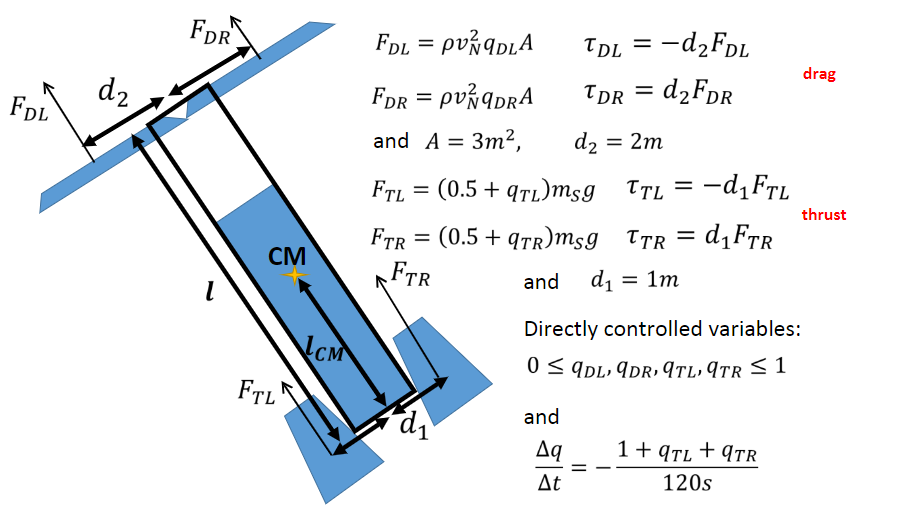
Inspired by the vertical landing of the SpaceX rockets, I created a 2D model of a rocket landing from high speed at orbit. This simulation included a model of the atmosphere for temperature and pressure, and included four point of control on the rocket - two thrusters and two drag flaps - as well as a limited amount of fuel. This simulation was written in Mathematica using an iterative time loop which solved a series of differential equations derived from classical physics. The full program can be found here.
Model of rocket using the drag flaps and thrusters for control. Due to the limited computational overhead, the time step of this program was 0.01s, limiting the amount I could effectively control the rocket. This model represents the closest result to a controlled landing.
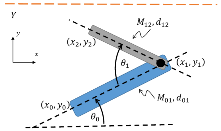
Another physical simulator was used to model and control a robot arm in microgravity trying to reach an oscillating target. For this simulator, I used Python to create a time loop and then solved a series of differential equations representing the physical model. At each step, I applied PD (proportional-derivative) control to move the arm closer to the target. The primary difficulty in this system was to control the angular momentum so that the arm does not spin out of control.
Animation of the simulated arm.
Trajectory plots of the arm.
Tension force in the muscle varies with attachment distance from shoulder, and the ideal curve changes depending on the angle of the arm.
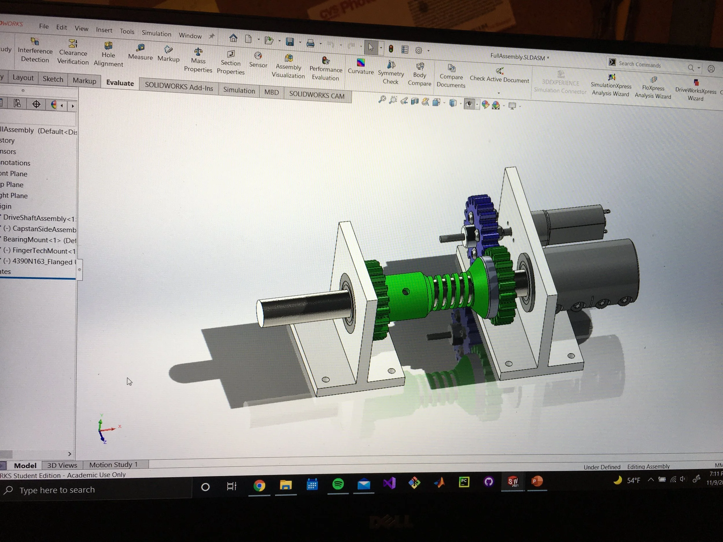
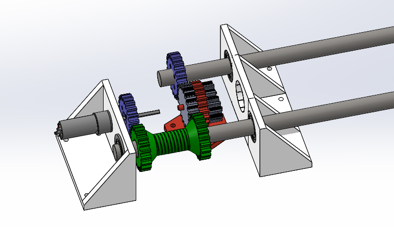
The purpose of this project was to develop a novel actuator systems based on capstan wrapping. In principle, the system is driven by one large motor, and the torque is distributed to several limbs by using capstans at each degree of freedom.
The capstans are engaged by small servo motors at each limb. This allows one large motor to drive the robot, and the capstans could engage and disengage around shafts to distribute the power. In theory, this allows each limb to be actuated with the full amount of torque provided by the main motor, and allows for a better strength-to-weight ratio for the whole system.
I designed the capstan mechanism at each joint of the robot, while advising and leading the team of undergraduates who built and tested the robot chassis.
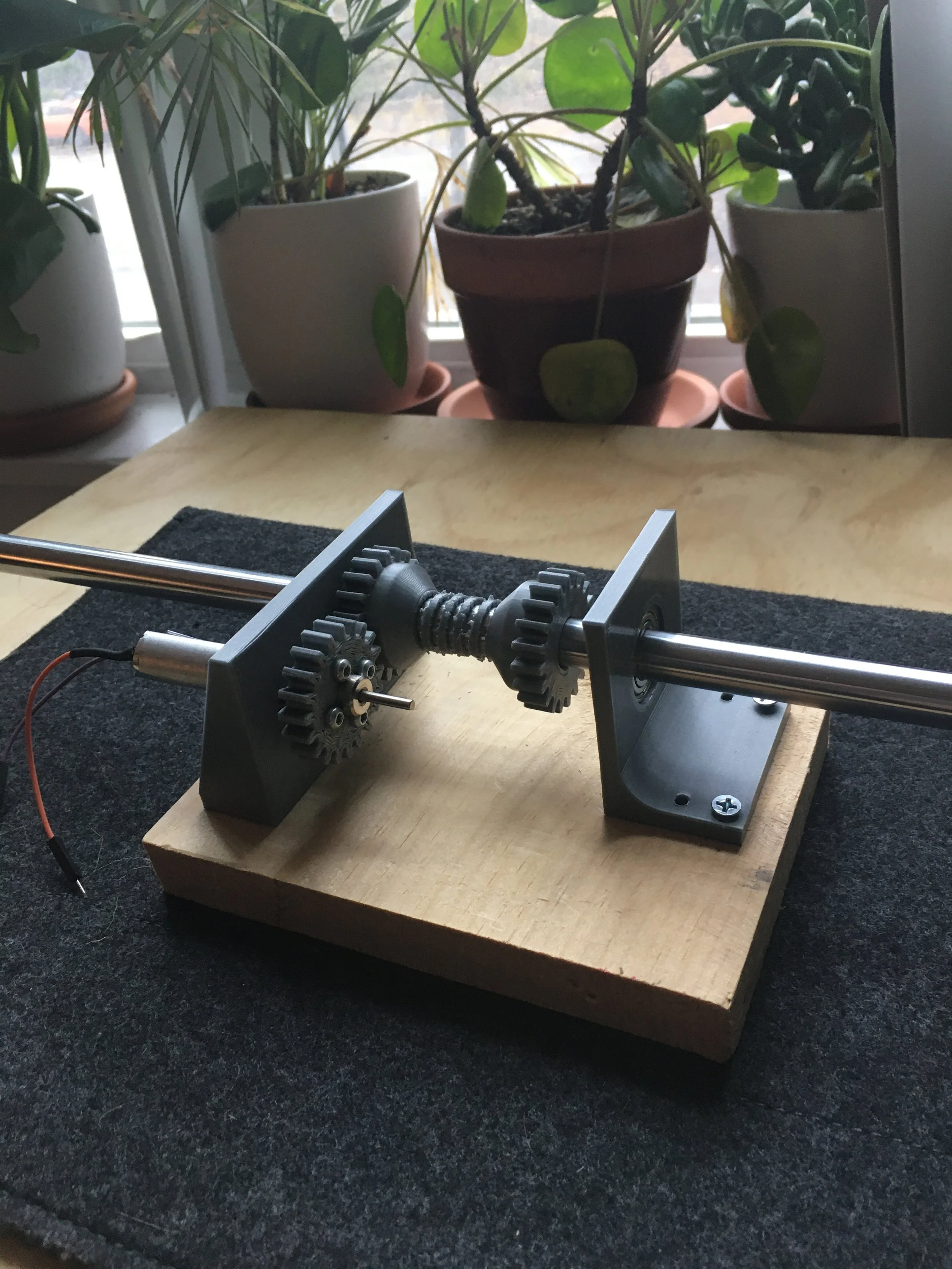
First version of the capstan mechanism design, placed at each joint of the robot. The shaft continuously rotates, driven by the main motor. To drive this degree of freedom, the small servo motor tightens the capstan around the shaft. The amount of friction provided by this tightening then drives the gear on the far side of the capstan and allows it to drive the limb.
Proof of concept for capstan engagement.
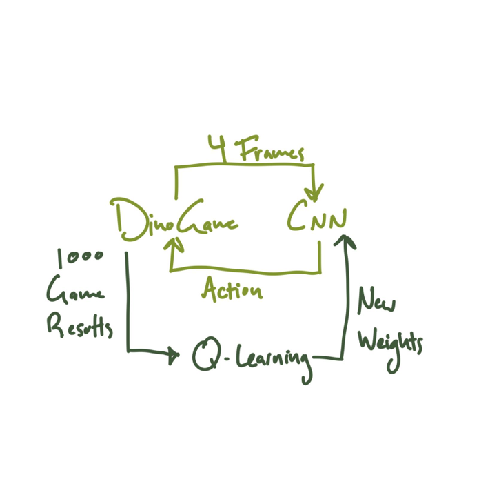
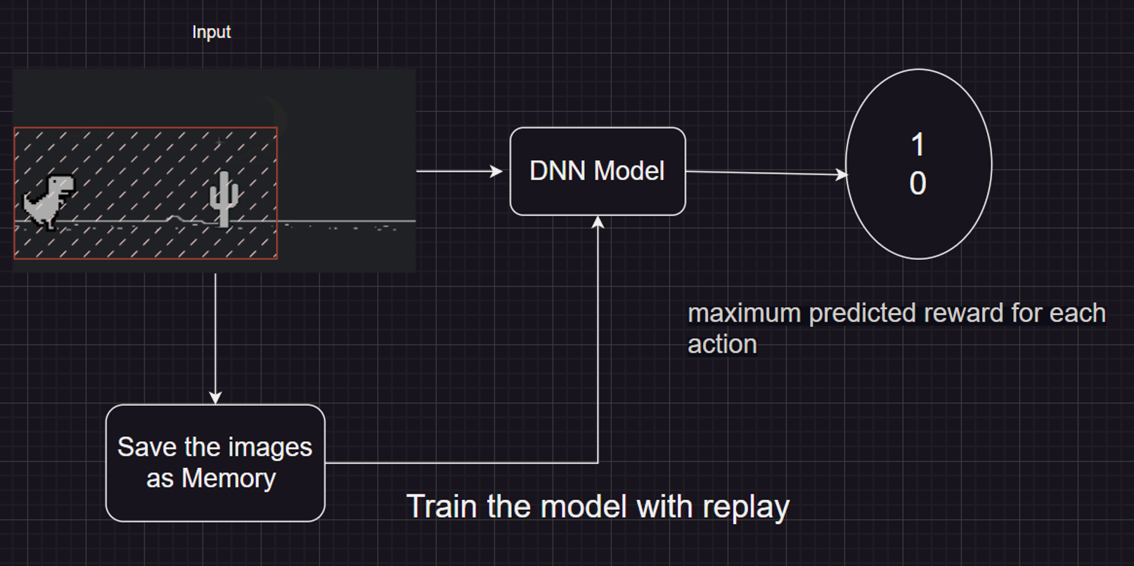
The goal of this project was to teach an agent to play the Google Chrome dinosaur jumping game using reinforcement learning. This project was completed for an Artificial Intelligence class.
The goal of the project was to show successful performance of a an agent trained using reinforcement learning to play the dino game (jumping and crouching to avoid obstacles).
The rough draft of the training architecture.
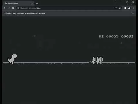
An early test of the dino game, still crashing into obstacle.
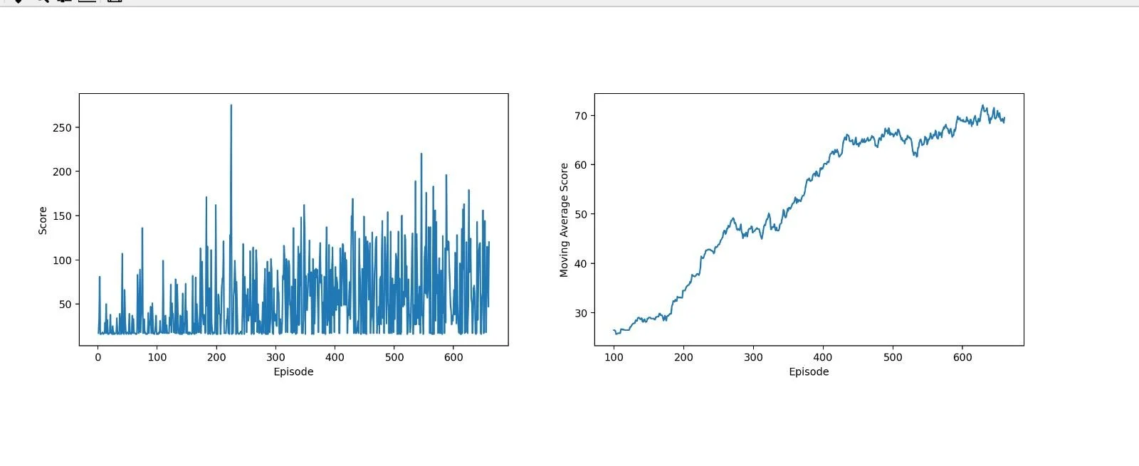
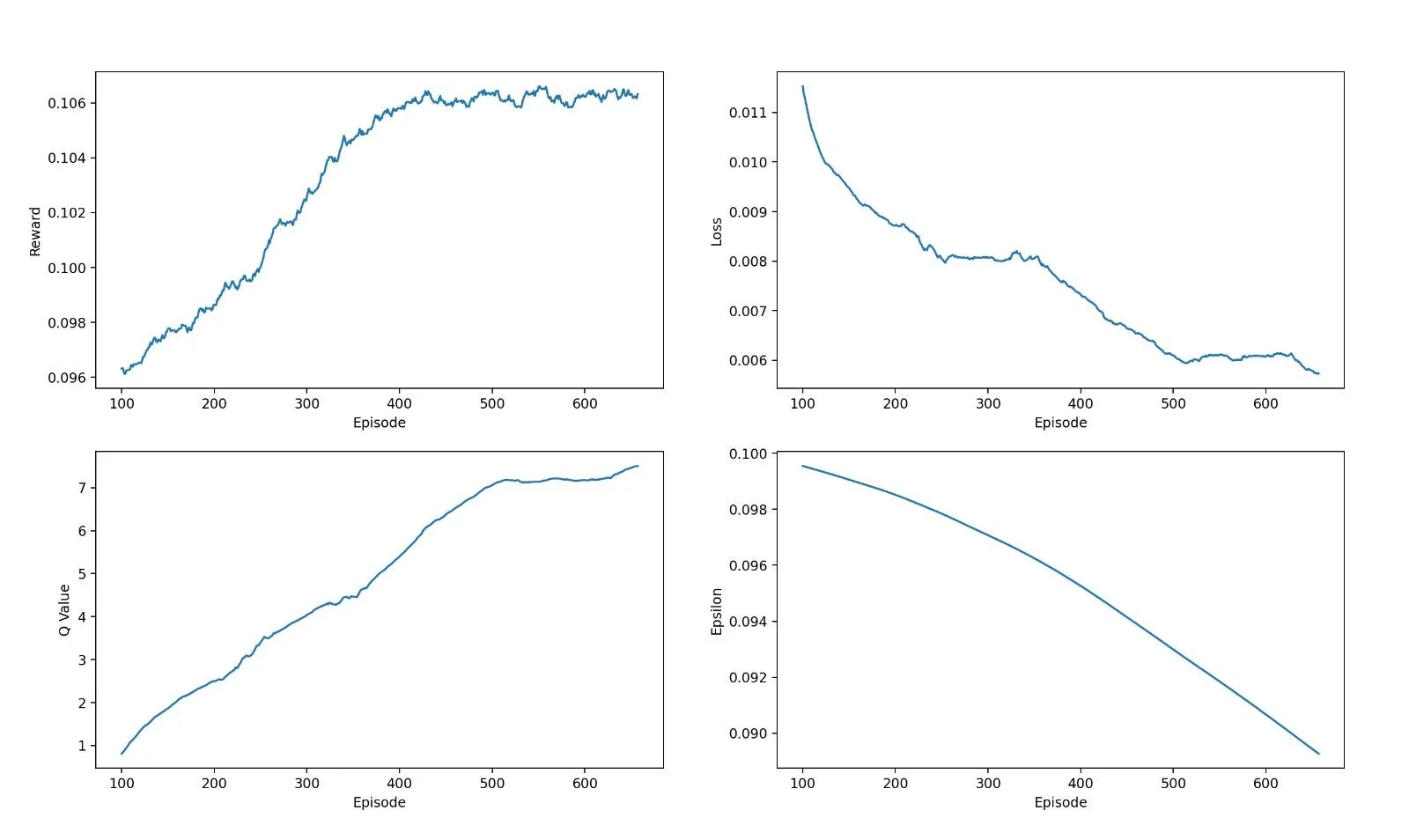
These plots show the improvement in score as the number of training episodes increased.
Training the learner overnight led to improved scores over over more training rounds.
The final results of the project show the reinforcement learner outperforming a human player (me).
Underwater robots are highly useful in performing tasks which are difficult or dangerous for a manned submersible craft and are becoming common in research and commercial applications. Autonomous underwater navigation has several challenging aspects including limited sensor data, maneuvering in a high density medium, and influences from tides and currents.
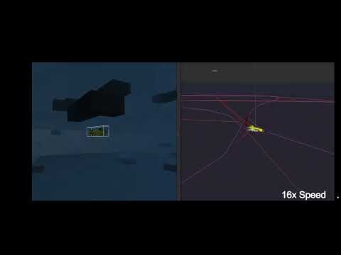
The goal of this project was to explore, and overcome, these challenges by creating a motion planning scheme for a simulated submarine-like-robot in an ocean environment with obstacles. The project resulted in the successful implementation of waypoint following by the ECA-A9 in a Gazebo simulation environment, the creation of a 3D world with modular obstacle settings, and the creation of an A* and Theta* path planning algorithm for the 3D case with Dubin’s path smoothing added post-generation.
Screen capture of the glider used for this project simulated in Gazebo
Diagram of the simulation architecture
Example of the randomly generated 3D obstacle field.
Example of a 3D path through the obstacle space